Gaussian Processes and Kriging

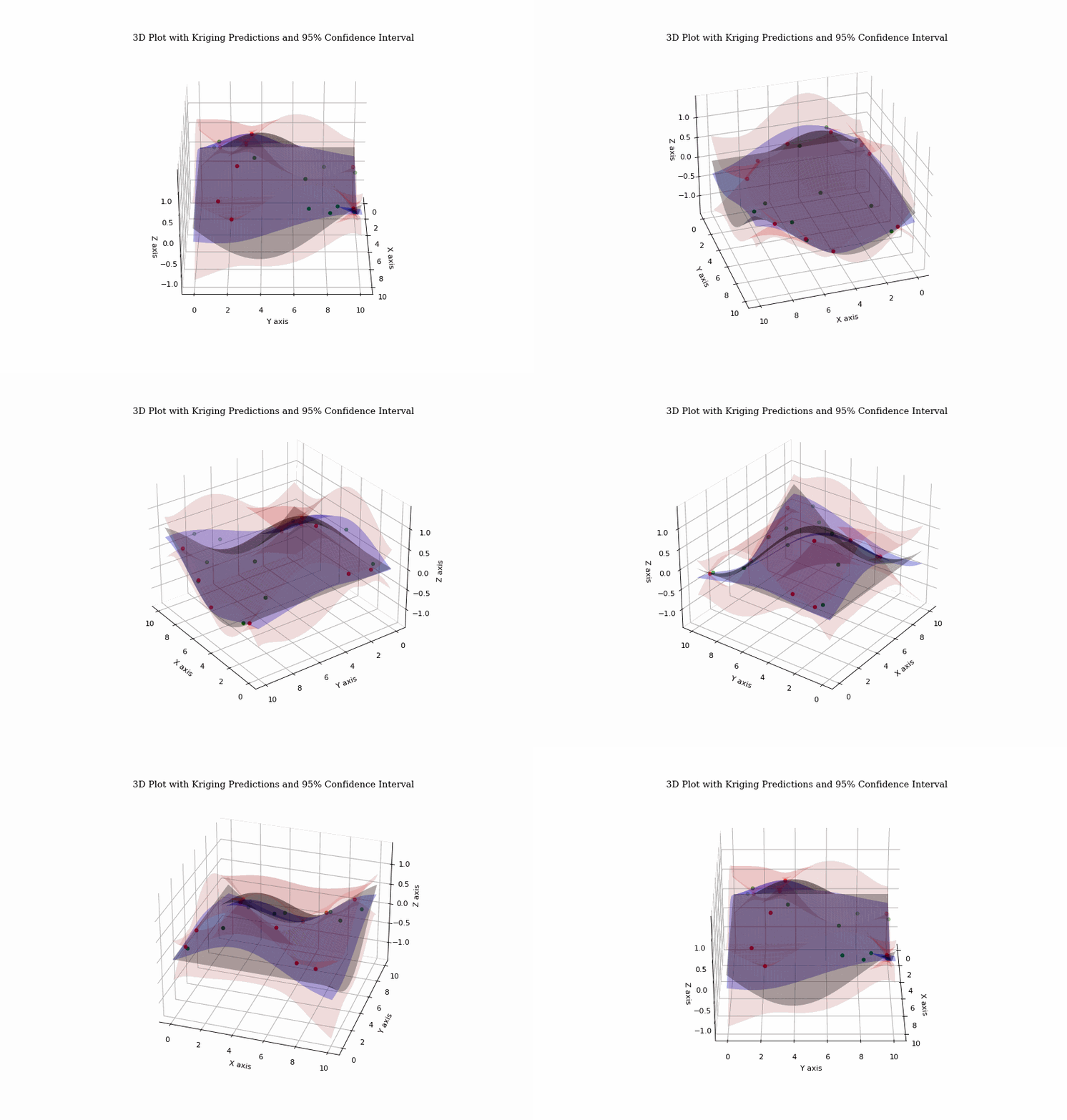
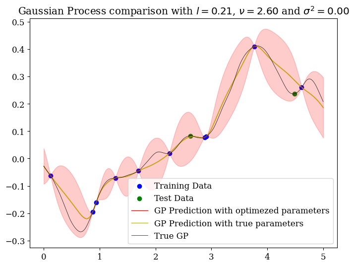
In this project, we implemented a Gaussian Processes and Kriging optimization based on Maximum Likelihood estimation of the parameters. We did it under the supervision of Pr Thierry Klein

Acces to report :

Report

Abstract

Gaussian processes are a fundamental tool in statistical learning with numerous applications, particularly in geostatistics. A Gaussian process is a stochastic process where any finite collection of random variables follows a multidimensional normal distribution, making it a powerful modeling tool.

Kriging, named after D.G. Krige, is a spatial prediction method leveraging Gaussian processes to interpolate unknown functions. There are two primary forms:

Simple Kriging: Assumes a constant, unknown mean.
Universal Kriging: Models the mean as a linear combination of known functions.

These methods provide optimal, unbiased estimates of a variable of interest using observed data, enabling predictions and conditional simulations. Conditional simulation generates realizations consistent with observations, aiding spatial uncertainty assessment and function reconstruction from partial or noisy data.

The covariance function is central to the regularity and continuity of Gaussian process trajectories. The kernel’s differentiability directly impacts trajectory properties. Estimating kernel parameters—via Maximum Likelihood or Cross Validation—optimizes kriging performance, enhancing prediction and simulation quality. This project focuses on these topics.

Keywords: Kriging, Gaussian Processes, Kernel Regularity, Maximum Likelihood Estimation, Geostatistical Interpolation.

2D function kriging with 95% confidence intervals

Introduction

Context and Motivation

Air pollution is a significant global health concern, causing nearly 6.7 million premature deaths annually (WHO). Understanding spatial air pollution levels within cities is vital, but large urban areas lack comprehensive measurement coverage.

Objective: Estimate air pollution levels throughout a city.
Approach: Kriging offers an effective solution for spatial interpolation with the following steps:

Collect data from monitoring stations across the city.
Analyze pollution variability with distance to identify an appropriate distance-pollution correlation.
Use kriging for interpolation and incorporate uncertainties to estimate error margins across city points.

This project highlights the implementation and exploration of Gaussian processes and kriging methods, emphasizing their practical application in geostatistical problems like urban air pollution mapping.

You can paste this into your website, and the Markdown formatting will render it appropriately.

Maximum Likelihood Estimation (MLE)

The likelihood function for a Gaussian process can be expressed as:

\[L(\sigma^2, \theta) := \frac{1}{n} \ln |\sigma^2 R_\theta| + \frac{1}{n} \frac{1}{\sigma^2} \mathbf{y}^t R^{-1}_\theta \mathbf{y}\]

Optimizing with respect to $\sigma^2$, for a fixed $\theta$, can be done explicitly. This reduces the dimensionality of the numerical optimization problem. The following proposition summarizes this result:

Proposition

The maximum likelihood estimator of $(\sigma^2, \theta)$ is $\hat{\sigma}^2_{ML}, \hat{\theta}_{ML}$, where:

\[\hat{\theta}_{ML} \in \arg\min_{\theta \in \Theta} L(\theta)\]

with:

\[L(\theta) = \ln(\hat{\sigma}^2_{ML}(\theta)) + \frac{1}{n} \ln |R_\theta|,\] \[\hat{\sigma}^2_{ML}(\theta) = \frac{1}{n} \mathbf{y}^t R^{-1}_\theta \mathbf{y},\]

and:

\[\hat{\sigma}^2_{ML} = \hat{\sigma}^2_{ML}(\hat{\theta}_{ML}).\]

Universal Kriging

For universal kriging, the mean function is no longer assumed to be zero. Let $H$ be the $n \times m$ matrix where:

\[H_{i,j} = g_j(x^{(i)}),\]

and the mean function is assumed to take the form:

\[\sum_{i=1}^m \beta_i g_i,\]

with known functions $g_i$ and unknown coefficients $\beta_i$. Let $h$ be the $m \times 1$ vector defined as:

\[h_j = g_j(x_{\text{new}}).\]

Explicitly incorporating $\sigma^2$ and $\theta$, we write the likelihood equations only for this case.

The likelihood criterion, depending on $\beta$, $\sigma^2$, and $\theta$, is:

\[L(\beta, \sigma^2, \theta) := \frac{1}{n} \ln |\sigma^2 R_\theta| + \frac{1}{n\sigma^2} (\mathbf{y} - H\beta)^t R^{-1}_\theta (\mathbf{y} - H\beta).\]

As with simple kriging, the likelihood criterion can be minimized explicitly with respect to $\beta$ and $\sigma^2$, eliminating $m + 1$ dimensions (the dimension of $\beta$ plus one). This is summarized in the following proposition:

Proposition

The maximum likelihood estimator of $(\beta, \sigma^2, \theta)$ is $(\hat{\beta}_{ML}, \hat{\sigma}^2_{ML}, \hat{\theta}_{ML})$, where:

\[\hat{\theta}_{ML} \in \arg\min_{\theta \in \Theta} L(\theta),\]

with:

\[L(\theta) = \ln (\hat{\sigma}^2_{ML}(\theta)) + \frac{1}{n} \ln |R_{\theta}|,\] \[\hat{\sigma}^2_{ML}(\theta) = \frac{1}{n} (\mathbf{y} - H\hat{\beta}_{ML}(\theta))^t R_{\theta}^{-1} (\mathbf{y} - H\hat{\beta}_{ML}(\theta)),\] \[\hat{\beta}_{ML}(\theta) = (H^t R_{\theta}^{-1} H)^{-1} H^t R_{\theta}^{-1} \mathbf{y},\]

and:

\[\hat{\beta}_{ML} = \hat{\beta}_{ML}(\hat{\theta}_{ML}),\\ \hat{\sigma}^2_{ML} = \hat{\sigma}^2_{ML}(\hat{\theta}_{ML}).\]

Additionally, we can express:

\[\hat{\sigma}^2_{ML}(\theta) = \frac{1}{n} \mathbf{y}^t \Pi_{\theta} \mathbf{y},\]

with:

\[\Pi_{\theta} = R_{\theta}^{-1} - R_{\theta}^{-1} H(H^t R_{\theta}^{-1} H)^{-1} H^t R_{\theta}^{-1}.\]

Important Example: The Matérn Kernel

To illustrate the previous theorem, we will use the Matérn kernel, a covariance matrix ($K$) that serves as a foundational tool for our research. The Matérn kernel is defined as follows:

\[K_{\text{Matern}}(d) = \sigma^2 \frac{2^{1-\nu}}{\Gamma(\nu)} \left( \frac{\sqrt{2\nu} \, d}{l} \right)^\nu K_\nu\left( \frac{\sqrt{2\nu} \, d}{l} \right)\]

Where the parameters are defined as:

$d$: The distance between two points. The kernel function must be decreasing with respect to $d$, as greater distances imply less influence between points.
$\sigma^2$: The variance of the kernel. A larger $\sigma^2$ corresponds to larger variations in the trajectories.
$l$: The length-scale parameter. Larger values of $l$ result in higher correlation between two points $x_1$ and $x_2$, effectively making the function smoother.
$\nu$: The regularity parameter. The function $Y$ is $k$-times differentiable in the least-squares sense and almost surely differentiable when $\nu > k$.

The Matérn kernel is crucial for our work as it balances flexibility and smoothness, making it ideal for modeling processes with varying levels of regularity and correlation.

Comparison of kriging with the true Matérn kernel and the one obtained through maximum likelihood estimation.

For more informations, refer to our Report.

@misc{Ebden2008,
  author = {M. Ebden},
  title = {Gaussian Processes for Regression: A Quick Introduction},
  month = {August},
  year = {2008}
}

@article{Bachoc2020,
  author = {F. Bachoc},
  title = {Asymptotic analysis of maximum likelihood estimation of covariance parameters for Gaussian processes: an introduction with proofs},
  institution = {Université de Toulouse},
  month = {September},
  year = {2020}
}

@misc{Wang2022,
  author = {J. Wang},
  title = {An Intuitive Tutorial to Gaussian Processes Regression},
  institution = {Queen’s University},
  month = {April},
  year = {2022}
}

@misc{Melo,
  author = {J. Melo},
  title = {Gaussian Processes for regression: a tutorial},
  institution = {University of Porto}
}

@article{BachocEtAl2017,
  author = {F. Bachoc and E. Contal and H. Maatouk and D. Rullière},
  title = {Gaussian processes for computer experiments},
  institution = {Institut de Mathématiques de Toulouse, ENS Cachan, INRIA Rennes, ISFA Université Lyon 1},
  year = {2017}
}

@misc{Breton2006,
  author = {J-C. Breton},
  title = {Processus Gaussiens, Master IMA 2ème année},
  institution = {Université de La Rochelle},
  month = {September-December},
  year = {2006}
}

@misc{Bachoc2020Notes,
  author = {F. Bachoc},
  title = {Lecture notes: Gaussian processes and sensitivity analysis for computer experiments},
  institution = {University Paul Sabatier},
  month = {January},
  year = {2020}
}

@misc{Krigeage,
  title = {Estimation paramétrique de la fonction de covariance dans le modèle de Krigeage par processus Gaussiens. Application à la quantification des incertitudes en simulation numérique}
}